A Resurgence of Neural Networks in Machine Learning
Today, we have a guest post from Dan Gillick, a Research Scientist at Google. He works on developing tools for automated natural language understanding, leveraging data at web scale to train large machine-learned models. Recent work has contributed to improvements in question answering and conversation search.
Prior to joining Google, Dan was a post-doctoral researcher at the International Computer Science Institute, studying speech recognition. He has a PhD from UC Berkeley in Computer Science and Bachelor’s degrees in Computer Science and English Literature from Wesleyan University. You can follow Dan on Google+ External link or on his website External link .
In graduate school, I spent a lot of time thinking about how to reduce “word error rate” (WER), the standard metric for assessing automatic speech recognition systems. The idea is to take recordings of all different people speaking all different kinds of stuff, get these recordings transcribed, usually by multiple people to reduce human error, and then count the number of words that an automatic system gets wrong.
In 2010, the best systems got around 25% WER for recorded phone conversations, meaning that a quarter of the words were misrecognized. This is actually pretty good, since people often speak very quickly with lots of background noise and add lots of disfluencies (e.g., “like…uh…yeah…so I…I…ok…right”). By comparison, the WER for Google Voice data, which includes search queries and dictated messages, was 16%.
Compared to other areas of artificial intelligence, speech is a mature field, especially since it was commercialized so early by IBM and Dragon Systems. Because of this, by the time 2010 rolled around, even incremental progress had become quite difficult. The four or five very best new ideas over the past few decades have yielded 5-10% improvements in the state of the art. Speech conferences include hundreds or even thousands of presentations on complex models that seem to work a bit better for one genre but not another. I decided to write my dissertation about an easier topic.
Then, right around 2011, strange new results turned up. Microsoft research reported a 30% improvement on conversational speech—reducing WER from around 25% to around 17%. Google reported a similar improvement on Voice data—from around 16% to around 12% WER. Speech researchers are a rather stoic bunch, but these numbers raised even the most jaded eyebrows. After all, they represented the single biggest improvement in 30 years!
The magic ingredient, it turned out, was really an old idea, dating back as far as the 1940s: neural networks. There’s really nothing magical about a neural network. It’s a natural extension of a simple linear model. Here, I’ll draw a picture:
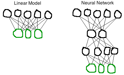
Image Caption: The image above features a linear model next to a neural network. The linear model features two rows of circles. The top row has five black circles and the bottom row has three green circles. Each circle in the top row is connected to each circle in the bottom row with a line. The neural network has four rows. The top row has five black circles, the second row has two black circles, the third row has four black circles and the fourth row has three green circles. Each circle in the first row is connected to each circle in the second row with a line. The pattern continues to the fourth row.
The top layer of circles are the numbers describing the input, sometimes called “features.” The features in a speech recognition model are measurements of the frequencies of the audio over a fraction of a second. The bottom layer of circles are the output. In a speech model, the outputs represent sub-word sounds like “ah” or “eh.” Each line is a “weight,” a number expressing the preference of each feature for each output. You can imagine 10 milliseconds of speech entering the model from the top, which causes the output sounds on the bottom to light up. The brightest is the most likely sound.
The neural network here has two “hidden” layers between input and output that represent intermediate features. These circles light up too as the input passes through, but the designer of the network has no particular expectation about what these intermediate features represent. The neural network’s architecture—its hierarchy of hidden layers—allows the model to represent layers of abstraction, from acoustic energy to auditory concepts, much like our brains appear to do. Through training, these increasingly abstract features emerge from the multi-layer structure. Actually, that is pretty magical.
In machine learning, “training” refers to the process of automatically choosing the weights given examples of the input where you know what the output should be. The basic idea is the same for both model varieties. Start by setting the weights to some random numbers. Pick up an example and pass it through the model. If the resulting output is not the same as the correct output, adjust the weights so the model will be closer to being correct the next time around. Just repeat this process over and over, passing through your training examples a bunch of times, until the weights aren’t changing much anymore.
The reason why it took so long to get neural networks to work better than linear models is that the details of the training process are tricky for neural networks. For both models, the goal is to find a set of weights (the lines in my pictures) that result in the model identifying as many training examples correctly as possible. Imagine each possible set of weights as a single point in a very high dimensional space. OK, this is pretty hard to imagine. But what’s important is that in the case of the linear model, all the points form a kind of high dimensional bowl. Training is like being a tiny explorer, where all you can see is the local landscape, trying to find the lowest point. Luckily, wherever you start out in a bowl, you can always get to the lowest point by walking down.
In the neural network case, you are not on a bowl. The landscape is much more complicated, filled with all kinds of peaks and valleys. It’s like you are trying to find Death Valley after being dropped blindfolded with no map into the middle of the Sierras. You can walk down, but you’ll probably end up in a muddy swamp thousands of feet higher up than the real lowest point.
There are many tricks researchers use to explore the space more efficiently, to try walking up before heading down again, but they require lots of training data (to better understand the landscape) and a huge amount of computation. One reason why success came a few years ago is that the specialized graphics cards built by video game developers for rendering extra-smooth 3D adventures can also be used to do the computations required for neural network training. Still, it takes weeks or even months to train one of these things.
All this progress in machine learning and in computation is pretty impressive. Still more impressive is that a baby’s brain learns a significantly better model for interpreting speech. It does this without any access to the underlying real words (labeled training examples). And, the total number of hours of speech Google uses to train its model is orders of magnitude more than the few thousand a child needs before fully comprehending language.
References:
Survey of Deep Neural Nets for Speech Recognition
Speech Recognition by Humans and Machines